Bulk RNA-seq & microarray
Understand each step.
See what changes.
Explore BulkSeq Studio in analysis order: from study design to biological interpretation. Each lesson shows what a setting changes and what it cannot establish.
Reproducible synthetic example
Experimental design
See when the model can separate the effects you ask it to estimate.
Full figure shown. Tap a mark to inspect values.
- Model
- Full rank
- Rank / columns
- 3 / 3
- Residual df
- 5
Full rank is necessary for estimation; it does not establish a sound biological design.
Focus the figure and use arrow keys, or select a mark, to inspect values.
Reproducible synthetic example
DESeq2 low-count prefilter
See which genes pass the count rule before DESeq2 model fitting.
Full figure shown. Tap a mark to inspect values.
- Eligible genes
- 450 / 480
- Required samples
- 4 Smallest condition group
- Minimum count
- 10 Per qualifying sample
Bars show 12 low-abundance examples; the count summarizes all input genes. This DESeq2 prefilter is separate from independent filtering of results. edgeR and limma-voom use design-aware filterByExpr, so their eligible genes can differ.
Focus the figure and use arrow keys, or select a mark, to inspect values.
Reproducible synthetic example
Normalization
Separate sequencing depth from composition effects.
Full figure shown. Tap a mark to inspect values.
- Gene
- N2
- Libraries
- 4
- Display
- Median ratio
One library doubles every count; another changes only N1. Inspect N2 to see how total scaling can spread a composition effect to an unchanged gene.
Focus the figure and use arrow keys, or select a mark, to inspect values.
Reproducible synthetic example
PCA and sample QC
Explore the sample variation captured by different feature sets.
Full figure shown. Tap a mark to inspect values.
- Genes used
- 100
- PC1 variance
- 72.6%
- PC2 variance
- 7.24%
The 20, 100, 450 gene settings are teaching examples. BulkSeq Studio defaults to 500 most variable genes, limited by retained genes. PCA is recomputed here for each set; separation is diagnostic, not a treatment-effect test. Axis signs are arbitrary.
Focus the figure and use arrow keys, or select a mark, to inspect values.
Reproducible synthetic example
Model fitting and shrinkage
Compare real method fits on the same simulated counts.
Full figure shown. Tap a mark to inspect values.
- Engine
- DESeq2
- Genes retained
- 450 Method-specific filtering
- Estimates
- Unshrunken
These are real fits on the same simulated counts, with each method’s filtering and normalization. Differences do not establish that one method is universally better.
Focus the figure and use arrow keys, or select a mark, to inspect values.
Precomputed synthetic DESeq2 run
Volcano plot
Full figure shown. Tap a point to inspect values.
Vertical axis: −log₁₀(adjusted p)
Cutoffs change selection; the model is not rerun.
- Below adjusted p cutoff
- 98 padj < 0.05
- Passing both
- 96 |log2FC| ≥ 1.00
- Higher / lower
- 52 / 44 in the displayed direction
Focus the plot, then use arrow keys to inspect synthetic examples one at a time. Home and End jump to the first and last examples.
Focus the figure and use arrow keys, or tap a point, to inspect values.
What this explains
Adjusted p-values account for multiple testing; they are not per-feature false probabilities.
Changing DESeq2’s alpha setting can reoptimize independent filtering during a run. This fixed example does not reproduce that process. Its fold-change slider is a post hoc screen, not a DESeq2 hypothesis test using lfcThreshold.
The comparison switch mirrors only this synthetic example. BulkSeq Studio preserves the comparison direction recorded in imported results.
Reproducible synthetic example
Expression heatmap
Explore within-gene patterns, displayed genes and colour limits.
Full figure shown. Tap a mark to inspect values.
- Genes displayed
- 8 Ranked by adjusted p
- Colour limit
- ±2.5 Row z-score
- Clipped cells
- 0 Original z-scores retained
Colour is relative within each gene, not absolute abundance across genes. BulkSeq clips row z-scores before Ward clustering, so changing the cap can also change ordering.
Focus the figure and use arrow keys, or select a mark, to inspect values.
Reproducible synthetic example
Enrichment
See why the eligible background changes an over-representation test.
Full figure shown. Tap a mark to inspect values.
- Selected features
- 10 Held fixed
- Background
- 100
- Sets tested
- 3 BH correction across all sets
Use eligible tested features mapped through the selected annotation route. The foreground, sets and overlaps are fixed here; larger dots mean more selected features overlap the set.
Focus the figure and use arrow keys, or select a mark, to inspect values.
Reproducible synthetic example
STRING association network
Filter displayed associations without changing the underlying evidence.
Full figure shown. Tap a mark to inspect values.
- Visible proteins
- 12
- Associations
- 19 Combined score ≥ 0.4
- Isolated proteins
- 0 At this display threshold
Scores illustrate STRING combined association evidence, not p-values or calibrated probabilities. Positions stay fixed; distance is not a biological quantity. Associations need not be direct physical binding. Filtering this saved example does not query STRING or recover omitted edges.
Focus the figure and use arrow keys, or select a mark, to inspect values.
About these examples
These examples use simulated counts and controlled synthetic examples, not a biological study. DESeq2, edgeR, limma-voom and apeglm results were computed in advance with the installed analysis packages. They are not fitted in your browser.
Heatmaps and PCA use the saved rlog sample matrix; the transformation is recorded with the fitted example. Heatmaps use within-gene sample-standard-deviation z-scores, symmetric clipping before Euclidean/Ward clustering, and trees recalculated for each displayed state; PCA centres the selected genes without variance-scaling them. Results-only imports cannot recreate these sample-level figures.
Network scores and gene sets are synthetic teaching examples. The edge scores illustrate combined association confidence, not interaction strength or a probability of direct binding. A STRING association can reflect physical, functional or regulatory relationships, and network layout is not a biological distance. STRING interpretation · DESeq2 methods
Choose your starting point.
Public accessions
Start with a public RNA-seq study and follow the read-to-results route.
- 1Prepare inputFetch public metadata
- 2Process readsChoose read processing
- 3Fit modelDefine the comparison
- 4Explore resultsRead and export results
No read-processing stage is skipped; the workflow first retrieves the reads.
View the stepsExplore the result.
Plots
Differential-expression figures and sample-level views, where your route supports them.
Enrichment & networks
Gene sets and interactive protein relationships.
Tables & provenance
Results, settings and checks in one record.
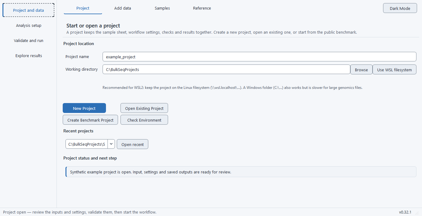
View the desktop interface
Handbook
Version 0.34.0
Get BulkSeq Studio.
Install the app, then prepare its analysis environment.
Installation guide ↗Analysis runs locally. Setup, public-data retrieval and online annotation services require connectivity.
For bulk-expression research, not single-cell analysis or clinical diagnosis. Review the study design, checks and interpretation with each result.